Designing the Base

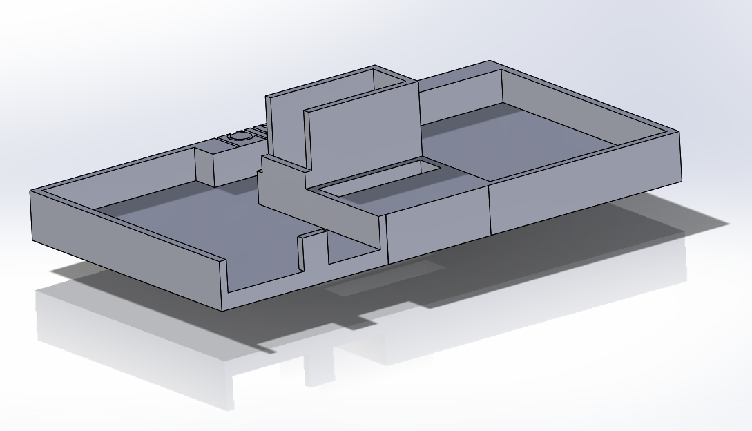
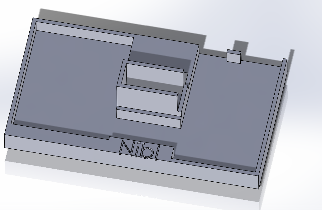
Our base design contains an area for the BeagleBone Blue, a breadboard, the servo for spinning the entire base, and the servo that changes the launch angle.

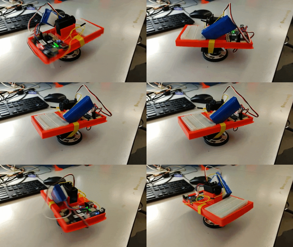
We got that printed the next morning, and fired up the servos! We had to file the breadboard and dremel the print to get it to fit, and we miiight have forgotten a place to put the battery. But we’re spinning and feeling good.

Playing with Voice Recognition

MFCC

As for voice recognition, we decided to prototype what we’ll finally implement on the MCU in Python on a laptop. Now, we probably don’t want to do the voice recognition the ESE 224 way. That is:

• Take an FFT of an input signal
• Dot it with a whole lot of labeled sample FFTs
• Find the highest dot product, and assign the input signal that label.

The weaknesses of this method are:

• Very specific to one voice
• Requires a huge amount of data and comparing
• Not good at identifying a signal that’s just noise.

We scoured the internet for ways to do light-weight voice recognition. What we settled on is called MFCC: Mel Frequency Cepstrum Coefficients. MFCC is a way to break down a signal into coefficients that represent how much of the energy of the signal resides in different frequency ranges (designed to mimic the human cochlea!). The best resource we found was from Practical Cryptography. The procedure is comically involved. Here are the Sparknotes:

• Filter the input signal
• Multiply it by a cosine
• Take the real coefficients of the FFT of the signal (aka DCT)
• Calculate the power periodogram of the FFT
• Make a series of 26 triangular filters based on Mel frequencies (which correspond to sensivity of the human ear), then convert back to the normal frequency domain
• See how much energy lies in each of those triangular filters
• Take the log all those energies
• Then take the DCT of all those energies
• Just throw out the last 14
• Finally, we have just 12 numbers to represent our signal

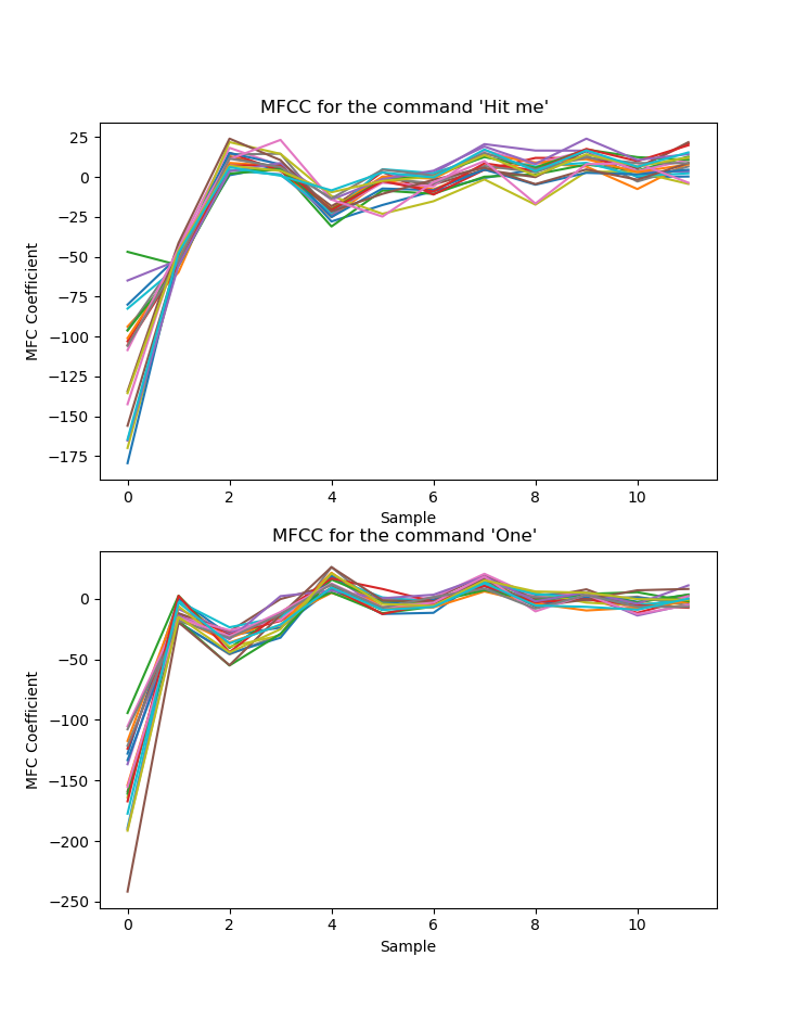
Why go through all this trouble? I want to reemphasize the last point. If we sample at 8000 Hz, and take a 1 second window, then our input signal is represented with 8000 numbers. MFCC reduces the dimensionality of this classification problem from 8000 to 12. Wow. Check out the different characteristic peaks in MFCC plots of two commands.

Classification

Now that we these 12 numbers, how do we identify what kind of command was recorded? We recorded a test set of 4 different sounds:

• “Hit me”
• “One”
• “Two”
• Just background noise

We then used a classification algorithm called quadratic discriminant analysis (QDA). If you’re interested in QDA, see this resource from SciKit. To perform QDA, all we’d need to store on the microcontroller would be some mean vectors and covariance matrices. The covariance matrices would be 12x12 for every output class. Way better than storing dozens of FFT vectors of length 8000!

Results

What happened next was pretty remarkable. At around six in the morning, we finally ran our test. We didn’t believe the results at first. We recorded a test set of 80 samples, 20 of each class (garbo refers to background noise). We used 3/4 of that for training and 1/4 for validation. Here’s the printout.

On training data, the results are:
Correct hit mes, Missed hit mes:17, 0
Correct ones, Missed ones:16, 0
Correct twos, Missed twos:13, 0
Correct garbo, Missed garbo:14, 0

On test data, the results are:
Correct hit mes, Missed hit mes:3, 0
Correct ones, Missed ones:4, 0
Correct twos, Missed twos:7, 0
Correct garbo, Missed garbo:6, 0

QDA correctly identified every sample in our test set. Granted, these tests were in quiet conditions, done with one voice, and recorded close to the mic. Nevertheless, when we record an additional sample and have it classify on the spot, it guesses right for either of our voices! There’s still work to do. But we’re very pleased with this start. We think with a bigger test set recorded in more realistic conditions, QDA and MFCC will be a winning combination.